Softmax 回归
概要
-
说是回归,解决的问题大多是分类问题
-
多输出,可以对应多分类
-
回归通常是单输出,预测某一个值
分类

回归
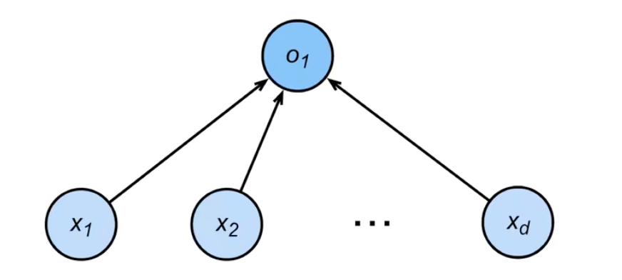
其中每一个箭头线代表一个权重 $w_{ij}$
都可以看作单层神经网络
开销
Softmax 中间输入层到输出层是全连接的,称其为 全连接层,说白了就是把输入和输出全用权重 $\mathbf{w}$ 关联起来
全连接层的参数开销通常非常大,如果有 $d$ 个输入和 $q$ 个输出,全连接层需要学习的参数有 $d * q$ 个这么多,参数开销记为 $O(dq)$
对于不是全连接层,从 $d$ 个输入到 $q$ 个输出可以引入一个超参数 $n$,使得参数开销降低为 $O(\frac{dq}{n})$
logistic 回归
可以理解成 Softmax 只有两个输出的特殊情况,这时这两个输出进行分类的话肯定一个是 1 一个是 0,对应逻辑(logistic)输出
Softmax 函数
将一个分布映射到 [0, 1] 的区间上,使其相加为 1 (概率分配)
$$ \mathbf{\hat{y}} = softmax(\mathbf{o}) $$
$\mathbf{o}$ 为输出向量
其中 $\hat{y}i$ 为: $$ \hat{y} {i} = \frac{\exp \left(o_ {i}\right)} {\sum_ {k}^{n} \exp \left(o_ {k}\right)} $$
使用指数的好处可以将原来分布里面的负数 $o_i$ 转换成正数 $\hat{y}_i$
缺点
-
softmax 很难将一个分布逼近到一个只有一个元素为 1 的剩余元素全为 0 的向量
假设 $\hat{y}_i$ 是需要逼近到 1 的元素
有 $\hat{y}_ {i}=\frac{\exp \left(o_ {i}\right)}{\sum_ {k}^{n} \exp \left(o_ {k}\right)}=1$
$\Leftrightarrow exp(o_i) = \sum_{k}^{n}exp(o_k)$
$\Leftrightarrow exp(o_1) + exp(o_2) + ... + exp(o_{i-1}) + exp(o_{i+1}) + ... + exp(o_{n}) = 0$
$exp(x) > 0$ 恒成立,只有当 $o_k$ 是一个绝对值很大的负数时才会逼近 $exp(o_k)$ 0
通常的解决方法是让它逼近一个 [0, 0, 0.9, ....] 类似的向量
-
softmax 处理的输入如果很大时,指数函数的暴增性可能会导致数值溢出,则需要将 $o_k - max(\mathbf{o})$ 定义为新的 $\hat{o}_k$
损失函数
在衡量两个分布的相似度时,在深度学习中常常使用
交叉熵损失 (cross-entropy loss)
信息论基础通俗理解
- 信息熵
公式 $$ H(p) = \sum_{i=1}^{n} p_klog(\frac{1}{p_k}) = -\sum_{i=1}^{n} p_klogp_k $$
其中 $p_k$ 是真实分布
信息熵作用是量化一个随机事件(一个概率分布)的不确定性
如果我们需要确定这个概率事件,即把不确定性降低为 0
比如买中彩票中大奖,我们需要最少买多少次彩票(最少花多少钱),才能把中奖这一个事件的不确定性降低为 0
这时候 最少买多少次彩票(最少花多少钱) 就等于信息熵的大小
再比如计算机压缩文件中,量化 预测所有字符 这一个事件(一个概率分布)的不确定性时,也可以引入信息熵
此时确定这个概率事件,即把文件记录下来(压缩文件),我们最少需要等同信息熵大小的数据量(单位那特(nat), $1 nat = \frac{1}{ln(2)} bit \approx 1.44 bit$ 信息熵计算是以 e 为底数的,2表示二进制编码)
例如有一个已知大小的文件,内容有 $\frac{1}{2}$ 的可能性全部是 0,有 $\frac{1}{2}$ 的可能性全部是 1,信息熵 $H(p) = \frac{1}{2}log_22 + \frac{1}{2}log_22 = 1$ (其中使用 2 为底数表示使用二进制编码),那么就需要 1 bit来记录这个文件,即 0 表示这个文件是全 0,1 表示这个文件是全 1
- 交叉熵 (cross entropy)
公式 $$ H(p,q) = \sum_{i = 1}^{n} p_ klog(\frac{1}{q_k}) = -\sum_ {i=1}^{n} p_ klog(q_ k) $$
其中 $p_k$ 是真实分布,$q_k$ 是预测分布
衡量一个非真实分布的不确定性时,就要引入交叉熵的概念
交叉熵等于使用预测分布的平均编码长度,相对使用真实分布得到的信息熵,交叉熵总是比信息熵要大,当且仅当预测分布等于真实分布时,交叉熵等于信息熵
所以交叉熵可以衡量与信息熵的接近大小,但最小时不是 0,而是信息熵的大小
最小化交叉熵,即使交叉熵无限接近信息熵(预测分布逼近真实分布),这可以作为机器学习中的损失函数来度量预测结果,进而优化模型
- 相对熵 (relative entropy) 也叫 KL散度 (Kullback–Leibler divergence)
公式 $$ KL(p,q) = \sum_{i=1}^{n} p_klog(\frac{1}{q_k})) - \sum_{i=1}^{n} p_klog\frac{1}{p_k} $$
其实就是交叉熵减去信息熵
用来衡量两个分布的接近大小
机器学习中一般不使用相对熵来优化模型,因为通常来说真实分布是确定的,那信息熵就是个定值,最小化相对熵就是在最小化交叉熵
KL散度是不对等的,即 $KL(p,q) ≠ KL(q, p)$ KL散度需要明确什么是真实分布,什么是预测分布
交叉熵损失函数
公式 $$ loss(\mathbf{y}, \mathbf{\hat{y}}) = -\sum_{i=1}^{n} y_ i log(\hat{y}_ i) $$
其中 $\mathbf{y}$ 是真实分布,$\mathbf{\hat{y}}$ 是预测分布
- 求导
$$ \operatorname{loss}(\mathbf{y}, \hat{\mathbf{y}})=-\sum_{i = 1}^{n} y_{i} \log \hat{y}_ {i} = -\sum _ {i = 1}^{n} y_ {i} \log \frac{\exp \left(o_ {j}\right)}{\sum_ {k = 1}^{n} \exp \left(o_{k}\right)} $$
$$ = \sum_{i=1}^{n}y_ilog\sum_{k=1}^{n}exp(o_k) - \sum_{i=1}^{n}y_io_j $$
在 softmax 分类问题中,真实分布是除了一个元素为 1(或者近似为1),剩余全是 0 的向量,而这里的 j 就是 1 所在真实分布向量里的索引位置
$softmax(\mathbf{o})_j = \hat{y}_j$ = 预测真实值的概率大小
接下来有 $$ loss(\mathbf{y}, \mathbf{\hat{y}}) = log\sum_{k=1}^{n}exp(o_k) - o_j $$ $$ \frac{\partial loss(\mathbf{y}, \mathbf{\hat{y}})}{\partial o_j} = \frac{exp(o_j)}{\sum_{k=1}^{n}exp(o_k)} - 1 $$ $$ = softmax(\mathbf{o})_j - 1 $$
其中 $y_j$ = 1,表示真实值概率为 1
这个导数就是预测的 $\hat{y}_j$ 和真实的 $y_j$ 的差
实现
使用 MNIST 数据集
import torch
import torchvision
from torchvision import datasets, transforms
from torch.utils import data
import matplotlib.pyplot as plt
import numpy as np

transform = transforms.ToTensor()

data_train = datasets.MNIST(root = "./data/",
                            transform=transform,
                            train = True,
                            download = True)

data_test = datasets.MNIST(root="./data/",
                           transform = transform,
                           train = False,
                           download = True)

len(data_train), len(data_test), data_train[0][0].shape
(60000, 10000, torch.Size([1, 28, 28]))
loader_train = data.DataLoader(dataset = data_train, batch_size = 100, shuffle = True)
loader_test = data.DataLoader(dataset = data_test, batch_size = 100, shuffle = True)

images, labels = next(iter(loader_train))
images.shape, labels.shape
(torch.Size([100, 1, 28, 28]), torch.Size([100]))
# 定义显示图片函数

def show_images(images, rows, colums, labels):
    img = torchvision.utils.make_grid(images, nrow=colums, ncolum=rows)
    img = img.numpy().transpose(1, 2, 0)
    plt.imshow(img)
    plt.show()
    print("labels: ", labels.reshape((rows, colums)))
show_images(images, 10, 10, labels)

    labels:  tensor([[0, 3, 1, 8, 7, 4, 2, 5, 9, 6],
            [4, 8, 0, 6, 8, 0, 8, 1, 1, 0],
            [1, 8, 4, 6, 2, 4, 9, 9, 6, 7],
            [3, 8, 3, 8, 4, 8, 4, 1, 9, 8],
            [1, 2, 4, 6, 3, 3, 1, 8, 5, 4],
            [3, 0, 4, 7, 1, 3, 2, 6, 1, 7],
            [6, 0, 7, 8, 7, 9, 3, 5, 2, 8],
            [7, 1, 7, 3, 4, 5, 5, 7, 1, 8],
            [5, 4, 5, 4, 8, 7, 4, 3, 5, 9],
            [7, 4, 8, 3, 6, 7, 4, 1, 4, 5]])
num_input = 28 * 28
num_output = 10

# 定义权重和偏差
W = torch.normal(0, 0.01, size=(num_input, num_output), requires_grad=True)
b = torch.zeros(num_output, requires_grad=True)
# 定义 softmax
def softmax(O):
    # 减去最大值防止数值溢出
    O -= O.max(1, keepdim=True)[0]
    O_exp = torch.exp(O)
    partition = O_exp.sum(1, keepdim=True)
    return O_exp / partition
# 测试一下
Y = softmax(torch.arange(16).reshape((4, 4)))
Y, Y.sum(1)
    (tensor([[0.0321, 0.0871, 0.2369, 0.6439],
             [0.0321, 0.0871, 0.2369, 0.6439],
             [0.0321, 0.0871, 0.2369, 0.6439],
             [0.0321, 0.0871, 0.2369, 0.6439]]),
     tensor([1., 1., 1., 1.]))
# 定义网络
def net(X):
    return softmax(torch.matmul(X.reshape((-1, W.shape[0])), W) + b)


# 交叉熵损失
# y_hat 是 batch_size rows, 10 columns 的矩阵
def cross_entropy(y_hat, y):
    return - torch.log(y_hat[range(len(y_hat)), y])


# 返回预测正确的样本数
def accuracy(y_hat, y):
    if len(y_hat.shape) > 1 and y_hat.shape[1] > 1:
        y_hat = y_hat.max(axis=1)[1]
    cmp = y_hat.type(y.dtype) == y
    return float(cmp.type(y.dtype).sum())

# 测试
# y_hat = torch.tensor([[0.2, 0.7, 0.1], [0.2, 0.3, 0.5]])
# y = torch.tensor([1, 1])
# cross_entropy(y_hat, y), accuracy(y_hat, y) / len(y_hat)

accuracy(net(images), labels) / len(labels) # 预测概率差不多等于随机猜
0.07
def sgd(param, lr, batch_size):
    with torch.no_grad():
        param -= lr * param.grad
# 训练
W = torch.normal(0, 0.01, size=(num_input, num_output), requires_grad=True)
b = torch.zeros(num_output, requires_grad=True)

loss = cross_entropy
num_epochs = 10
lr = 0.012

l_train = []
a_train = []
a_test = []

for epoch in range(num_epochs):
    loss_epoch = []
    accuracy_train_epoch = []
    accuracy_test_epoch = []

    for X, y in loader_train:
        l = loss(net(X), y)
        # 梯度清零
        if W.grad is not None:
            W.grad.zero_()
            b.grad.zero_()
        # 计算梯度
        l.sum().backward()
        # 更新参数
        sgd(W, lr, len(y))
        sgd(b, lr, len(y))

        loss_epoch.append(loss(net(X), y).sum())
        accuracy_train_epoch.append(accuracy(net(X), y) / len(y))

    for X_test, y_test in loader_test:
        accuracy_test = accuracy(net(X_test), y_test) / len(y_test)
        accuracy_test_epoch.append(accuracy_test)

    l = torch.tensor(loss_epoch).mean()
    a = torch.tensor(accuracy_train_epoch).mean()
    a_t = torch.tensor(accuracy_test_epoch).mean()

    print(f"loss {l} train data accuracy {a} test data accuracy {a_t}")
    l_train.append(l)
    a_train.append(a)
    a_test.append(a_t)
    loss 31.28058624267578 train data accuracy 0.9169498682022095 test data accuracy 0.8971999287605286
    loss 21.3648738861084 train data accuracy 0.9435666799545288 test data accuracy 0.9202000498771667
    loss 20.323776245117188 train data accuracy 0.9458498954772949 test data accuracy 0.9225000143051147
    loss 20.020654678344727 train data accuracy 0.9476000070571899 test data accuracy 0.9214000105857849
    loss 19.555438995361328 train data accuracy 0.947916567325592 test data accuracy 0.9117000699043274
    loss 19.459369659423828 train data accuracy 0.9493000507354736 test data accuracy 0.9197999835014343
    loss 19.1043643951416 train data accuracy 0.9503500461578369 test data accuracy 0.9086999297142029
    loss 18.949724197387695 train data accuracy 0.9509999752044678 test data accuracy 0.9083000421524048
    loss 18.79474639892578 train data accuracy 0.9518333077430725 test data accuracy 0.9097999334335327
    loss 18.816661834716797 train data accuracy 0.9512166380882263 test data accuracy 0.9115000367164612
plt.plot(np.arange(1, num_epochs+1), np.array(l_train) / np.max(l_train))
plt.plot(np.arange(1, num_epochs+1), np.array(a_train))
plt.plot(np.arange(1, num_epochs+1), np.array(a_test))
plt.show()

- 训练精度达到 0.95 后很难再上升 (softmax 很难逼近 1 这种情况)
- 验证数据集精度稍微比训练数据集低一点
- 精度难以再提升一部分原因是把图像拉成向量会损失图像的平面信息
X_test, y_test = next(iter(loader_test))
y_hat = net(X_test)
y_hat = y_hat.max(axis=1)[1]
# 展示验证数据集图片和预测值
show_images(X_test, 10, 10, y_hat.type(y.dtype))
accuracy(net(X_test), y_test) / len(y_test)

    labels:  tensor([[7, 1, 8, 1, 2, 0, 5, 5, 9, 4],
            [8, 5, 4, 9, 9, 6, 8, 9, 7, 2],
            [6, 6, 1, 1, 2, 2, 2, 9, 5, 4],
            [9, 3, 3, 8, 1, 4, 2, 4, 1, 9],
            [2, 5, 4, 5, 4, 5, 1, 6, 9, 6],
            [6, 9, 8, 4, 3, 8, 4, 7, 3, 4],
            [6, 7, 7, 2, 2, 3, 1, 3, 4, 8],
            [0, 4, 1, 0, 2, 4, 5, 3, 1, 5],
            [5, 3, 3, 3, 4, 6, 7, 4, 9, 1],
            [4, 7, 9, 1, 6, 8, 6, 2, 3, 8]])

    0.88
images, labels = next(iter(loader_train))
y_hat = net(images)
y_hat = y_hat.max(axis=1)[1]
# 展示训练数据集图片和预测值
show_images(images, 10, 10, y_hat.type(y.dtype))
accuracy(net(images), labels) / len(labels)

    labels:  tensor([[0, 9, 1, 3, 5, 5, 1, 2, 8, 7],
            [0, 8, 6, 8, 9, 6, 9, 5, 7, 1],
            [1, 1, 2, 7, 3, 6, 7, 3, 8, 6],
            [6, 1, 4, 0, 1, 4, 1, 9, 7, 9],
            [6, 5, 2, 7, 6, 8, 3, 4, 2, 6],
            [6, 0, 8, 5, 4, 6, 1, 2, 1, 9],
            [7, 8, 9, 2, 0, 1, 5, 4, 4, 3],
            [7, 3, 5, 6, 2, 7, 1, 0, 3, 7],
            [1, 5, 7, 1, 3, 7, 3, 0, 0, 3],
            [0, 5, 6, 6, 8, 0, 2, 5, 9, 3]])

    0.93
pytorch 实现
from torch import nn

# 使用 flatten 展平层展平输入
net = nn.Sequential(nn.Flatten(), nn.Linear(num_input, num_output))

def init_weights(m):
    if type(m) == nn.Linear:
        nn.init.normal_(m.weight, std=0.01)

# 初始化权重
net.apply(init_weights)
    Sequential(
      (0): Flatten(start_dim=1, end_dim=-1)
      (1): Linear(in_features=784, out_features=10, bias=True)
    )
loss = nn.CrossEntropyLoss()

num_epochs = 10

# 学习率得调高点,不然跑不动
lr = 1

trainer = torch.optim.SGD(net.parameters(), lr=lr)

l_train = []
a_train = []
a_test = []

def train(net, trainer):
    l_train.clear()
    a_train.clear()
    a_test.clear()
    for epoch in range(num_epochs):
        loss_epoch = []
        accuracy_train_epoch = []
        accuracy_test_epoch = []

        for X, y in loader_train:
            l = loss(net(X), y)
            # 梯度清零
            trainer.zero_grad()
            # 计算梯度
            l.backward()
            # 更新参数
            trainer.step()

            # 评价模型对训练数据集的精度
            loss_epoch.append(loss(net(X), y).sum())
            accuracy_train_epoch.append(accuracy(net(X), y) / len(y))

        # 评价模型对验证数据集的精度
        for X_test, y_test in loader_test:
            accuracy_test = accuracy(net(X_test), y_test) / len(y_test)
            accuracy_test_epoch.append(accuracy_test)

        l = torch.tensor(loss_epoch).mean()
        a = torch.tensor(accuracy_train_epoch).mean()
        a_t = torch.tensor(accuracy_test_epoch).mean()

        print(f"loss {l} train data accuracy {a} test data accuracy {a_t}")
        l_train.append(l)
        a_train.append(a)
        a_test.append(a_t)

train(net, trainer)
    loss 0.2938828468322754 train data accuracy 0.9204166531562805 test data accuracy 0.9133999347686768
    loss 0.21709856390953064 train data accuracy 0.9428834319114685 test data accuracy 0.9127998948097229
    loss 0.2074650526046753 train data accuracy 0.9461498856544495 test data accuracy 0.9208000302314758
    loss 0.20276999473571777 train data accuracy 0.9473833441734314 test data accuracy 0.9202998876571655
    loss 0.19982706010341644 train data accuracy 0.9477667212486267 test data accuracy 0.9177000522613525
    loss 0.19807247817516327 train data accuracy 0.9492833614349365 test data accuracy 0.921999990940094
    loss 0.1955501288175583 train data accuracy 0.9491166472434998 test data accuracy 0.9122000336647034
    loss 0.1937972456216812 train data accuracy 0.9501833319664001 test data accuracy 0.9212000370025635
    loss 0.19263283908367157 train data accuracy 0.9512999653816223 test data accuracy 0.9132999181747437
    loss 0.1911425143480301 train data accuracy 0.9507499933242798 test data accuracy 0.9160000085830688
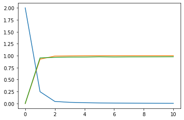
plt.plot(np.arange(0, num_epochs+1), np.array([2.] + l_train))
plt.plot(np.arange(0, num_epochs+1), np.array([0.] + a_train))
plt.plot(np.arange(0, num_epochs+1), np.array([0.] + a_test))
plt.show()

- 和自己实现的一样,单全连接层训练数据集精度达到 0.95 就很难上升
引入多层感知机
# 一层

num_hidden = 256

# 使用 ReLU 激活函数
net = nn.Sequential(nn.Flatten(), nn.Linear(num_input, num_hidden), nn.ReLU(), nn.Linear(num_hidden, num_output))

net.apply(init_weights)

trainer = torch.optim.SGD(net.parameters(), lr=lr)

train(net, trainer)
    loss 0.2471616417169571 train data accuracy 0.9269665479660034 test data accuracy 0.9535000324249268
    loss 0.04308231547474861 train data accuracy 0.9921665191650391 test data accuracy 0.9653000831604004
    loss 0.024812132120132446 train data accuracy 0.9959833025932312 test data accuracy 0.9711999297142029
    loss 0.0169887263327837 train data accuracy 0.9979166388511658 test data accuracy 0.972100019454956
    loss 0.012059231288731098 train data accuracy 0.9987832903862 test data accuracy 0.9765000939369202
    loss 0.009093635715544224 train data accuracy 0.9990666508674622 test data accuracy 0.9737000465393066
    loss 0.0071004582569003105 train data accuracy 0.9993166327476501 test data accuracy 0.9754000902175903
    loss 0.005697827786207199 train data accuracy 0.9995166063308716 test data accuracy 0.9758000373840332
    loss 0.004697315860539675 train data accuracy 0.9996333718299866 test data accuracy 0.976300060749054
    loss 0.0038973120972514153 train data accuracy 0.9996667504310608 test data accuracy 0.9773000478744507
plt.plot(np.arange(0, num_epochs+1), np.array([2.] + l_train))
plt.plot(np.arange(0, num_epochs+1), np.array([0.] + a_train))
plt.plot(np.arange(0, num_epochs+1), np.array([0.] + a_test))
plt.show()
- 引入一个隐藏层后,线性模型变成了非线性
- 精度又得到了提升
- 训练精度比较高,似乎是模型记住了训练集了
# 多层

num_hidden_1, num_hidden_2, num_hidden_3 = (256, 64, 16)

# 使用 ReLU 激活函数
net = nn.Sequential(
    nn.Flatten(),
    nn.Linear(num_input, num_hidden_1), nn.ReLU(),
    nn.Linear(num_hidden_1, num_hidden_2), nn.ReLU(),
    nn.Linear(num_hidden_2, num_hidden_3), nn.ReLU(),
    nn.Linear(num_hidden_3, num_output)
)

net.apply(init_weights)

lr = 0.6

trainer = torch.optim.SGD(net.parameters(), lr=lr)

train(net, trainer)
    loss 2.195422410964966 train data accuracy 0.1589166671037674 test data accuracy 0.4745999872684479
    loss 0.4805268943309784 train data accuracy 0.8359333276748657 test data accuracy 0.9422999620437622
    loss 0.06110946834087372 train data accuracy 0.986266553401947 test data accuracy 0.9613999724388123
    loss 0.033248934894800186 train data accuracy 0.9929832220077515 test data accuracy 0.9620999693870544
    loss 0.022589070722460747 train data accuracy 0.9956833124160767 test data accuracy 0.9670000672340393
    loss 0.01711619459092617 train data accuracy 0.9965166449546814 test data accuracy 0.9688000679016113
    loss 0.0124347023665905 train data accuracy 0.9976165890693665 test data accuracy 0.9731000661849976
    loss 0.009303041733801365 train data accuracy 0.9982666969299316 test data accuracy 0.9743000268936157
    loss 0.007649140432476997 train data accuracy 0.9984999299049377 test data accuracy 0.9754999279975891
    loss 0.007560083642601967 train data accuracy 0.9984333515167236 test data accuracy 0.9738000631332397
plt.plot(np.arange(1, num_epochs+1), np.array(l_train))
plt.plot(np.arange(1, num_epochs+1), np.array(a_train))
plt.plot(np.arange(1, num_epochs+1), np.array(a_test))
plt.show()

- 三层感知机模型处理后精度反而比单层低一丢丢
可能是概率问题 也可能是三层学习到一些奇怪的特征对判断造成了影响
比如训练一个模型分类男性女性,三层模型发现训练集里戴眼镜的大多数是男性,不戴眼镜的大多数是女性 它把这些当作权重学习了可能会对精度造成影响
总结
- softmax 回归
- 交叉熵损失
- 图像的平面信息对于图像识别也很重要
- 模型的复杂度越高越容易过拟合