梯度下降/上升

import matplotlib.pyplot as plt
import numpy as np

X = np.linspace(-np.pi, np.pi, 256, endpoint=True)
C = np.cos(X)

plt.plot(X,C)

plt.show()

对于上面的一个凸函数，如何不知道函数的表达式，或者表达式难以求导 需要对其求最大值，可以使用梯度上升法一步一步沿着梯度求最大值

K = np.append((X*(X+1))[:64*3], (X*(X+1)-10)[64*3:])

plt.plot(X, K)
plt.show()

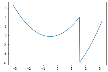
但对于某些奇怪的函数，例如上面，梯度下降可能会陷入局部最优解

• 梯度下降/上升也是属于一种贪心算法，容易陷入局部最优

步骤

1. 随机找一个初始值 $w _ 0$
2. 按照 $\mathbf{w} _ {t} = \mathbf{w} _ {t-1}-\eta \frac{\partial \ell}{\partial \mathbf{w} _ {t-1}}$ 来重复迭代参数t

其中 $\eta$ 是学习率, $ \frac{\partial \ell}{\partial \mathbf{w} _ {t-1}}$ 是 $loss$ 损失函数的梯度

Learning rate

简称 lr

• lr 是一个超参数，需要在训练模型之前定义

• lr 不能太大，也不能太小 (经典的超参数性质)

• 大了就步子迈大了，容易扯着蛋(

• 太小 epochs 得往上拉才能训练出一个合适的模型

合适的 lr

小批量随机梯度下降

• 结合批量梯度下降和随机梯度下降，是梯度下降算法中默认的求法
• 完整的跑一遍训练集代价太大
• 所以每次训练都随机从训练集中抽取小批量来训练，可以提升训练速度
• 随机采样 n 个样本 $i _ 1, i _ 2, i _ 3, ...., i _ n$，计算损失的平均值 $\frac{1}{n} \sum _ {i \in I _ n} \ell(\mathbf{x} _ i, y _ i, \mathbf{w})$

其中 n 也是一个超参数

n 不能太大，太大内存消耗更多，样本有一定概率相同的话，大批量会使得重复计算的可能性上升

n 不能太小，太小不适合GPU进行并行计算优化

优化

数据向量化

$\mathbf{w} _ {t}=\mathbf{w} _ {t-1}-\eta \frac{\partial \ell}{\partial \mathbf{w} _ {t-1}}$ 中 $\mathbf{w}$ 可以是影响 $loss$ 的一个标量参数，如果 $\mathbf{w}$ 可取 $\mathbf{w} _ 0, \mathbf{w} _ 1, \mathbf{w} _ 2,...,\mathbf{w} _ n$，可以将 $w$ 向量化成一个向量 $[\mathbf{w} _ 0, \mathbf{w} _ 1, \mathbf{w} _ 2,...,\mathbf{w} _ n]^T$

lr = 0.03
num_epochs = 5
grads = np.array([[2.0, 1.0], [0.7, 0.4], [0.3, 0.2], [0.2, 0.1], [-0.1,-0.02]])  # 这里直接写好了梯度

def sgd(w, grad):
    w -= lr * grad

w = np.array([1.0, 2.0])

for epoch in range(num_epochs):
    for i in range(len(grads)):
        sgd(w, grads[i])
        
    print(f"epoch {epoch + 1} :{w}")

    epoch 1 :[0.907  1.9496]
    epoch 2 :[0.814  1.8992]
    epoch 3 :[0.721  1.8488]
    epoch 4 :[0.628  1.7984]
    epoch 5 :[0.535 1.748]

获取随机小批量

import random

def data_iter(batch_size, features, labels):
    num_samples = len(features)
    indices = list(range(num_samples))
    # 打乱索引
    random.shuffle(indices)
    
    # 确保每个 epoch 都能扫到所有的训练数据
    for i in range(0, num_samples, batch_size):
        batch = np.array(indices[i:min(i + batch_size, num_samples)])
        features_batch = features[batch]
        labels_batch = labels[batch]
        # 加上 batch 大小并返回
        yield features_batch, labels_batch, len(batch)

batch_size = 10
features = np.random.normal(loc=0.0, scale=1.0, size=208).reshape(104, 2)
lables = np.random.normal(loc=0.0, scale=1.0, size=104)

features[:5]

    array([[ 0.73911935, -0.58917628],
           [-2.1565438 ,  1.47503143],
           [ 0.94866773, -0.85682476],
           [-0.18012857, -0.03176761],
           [ 0.21976216,  0.19298218]])

lables[:5]

    array([-0.95478689, -0.71763201,  0.25806049, -2.05750401, -1.51843728])

for X, y, l in data_iter(batch_size, features, lables):
    print(f"features_batch: {X[0]}, labels_batch: {y[0]}, batch_size: {l}")

    features_batch: [-1.45485397 -0.39236135], labels_batch: 0.12318386924794186, batch_size: 10
    features_batch: [-1.43973829  0.78538624], labels_batch: -0.8234640736033031, batch_size: 10
    features_batch: [0.30462236 0.07124829], labels_batch: 0.20986935899039746, batch_size: 10
    features_batch: [-0.37700071 -0.20652541], labels_batch: 2.3357916154234353, batch_size: 10
    features_batch: [-0.77891528 -0.9346586 ], labels_batch: -0.1957866052492824, batch_size: 10
    features_batch: [-0.40627378  0.2567436 ], labels_batch: 1.0447063842774422, batch_size: 10
    features_batch: [-0.23127423  0.01000124], labels_batch: -0.275188295527573, batch_size: 10
    features_batch: [-0.58167182 -3.57120846], labels_batch: 1.1866751115430718, batch_size: 10
    features_batch: [-1.49816488 -0.17920149], labels_batch: 0.6971271403274875, batch_size: 10
    features_batch: [-0.44691797  0.03166521], labels_batch: -0.8881366562785638, batch_size: 10
    features_batch: [-0.07057601  0.27185821], labels_batch: -1.0327701589004996, batch_size: 4

线性回归

主要从下面公式中求解出 $w$ 和 $b$

$y = x _ 0w _ 0 + x _ 1w _ 1 + ... + x _ {n-1}w _ {n-1} + b$

向量化后

$$ y = \begin{bmatrix} x_0 & x_1 & x_2 & ... & x_{n-1} & 1 \end{bmatrix}\begin{bmatrix} \mathbf{w} _ 0 \ \mathbf{w} _ 1\ \mathbf{w} _ 2\ ...\ \mathbf{w} _ {n-1}\ b \end{bmatrix} $$

抽象一下就是这样 $$ y = \left \langle \mathbf{X},\mathbf{w} \right \rangle $$

损失函数

$$ loss(\mathbf{X},\mathbf{y},\mathbf{w}) = \frac{1}{2n}\sum _ {i}^{n}(y _ i - \hat{y} _ i)^2 = \frac{1}{2n} \left |\mathbf{y}- \mathbf{X}\mathbf{w} \right |^2 $$

其中 $\hat{y}_i$ 是 预测值 $y_i$ 是 真实值

$\mathbf{X}$ 可以是矩阵，那么 $\mathbf{y}$ 就是向量，反之 $\mathbf{X}$ 是向量，那么 $\mathbf{y}$ 就是一个标量(数)

$\frac{1}{2n}$ 中 2 的作用是消除 L2 范数中平方导数后的影响

求导

• 对 $\mathbf{w}$ 求导

$$ \frac{\partial }{\partial \mathbf{w}} loss(\mathbf{X},\mathbf{y},\mathbf{w}) = \frac{\partial}{\partial \mathbf{w}} \frac{1}{2n} \left |\mathbf{y}- \mathbf{X}\mathbf{w} \right |^2 $$ $$ = - \frac{1}{n} (\mathbf{y} - \mathbf{Xw})^T \mathbf{X} $$

令其等于 0 求得极值点(如果有唯一解肯定是最优解点)

解得

$$ \frac{1}{n} (\mathbf{y} - \mathbf{Xw})^T \mathbf{X} = 0 \Longleftrightarrow \mathbf{w}^{*T} = \mathbf{y}^T\mathbf{X}(\mathbf{X}^T\mathbf{X})^{-1} $$

从以上推导可以看出

• 线性回归存在显示解

import numpy as np
import random
from matplotlib import pyplot as plt

true_param = np.array([2.6, -3.4, 4.2])  # 分别是 w_0, w_1, b

# 生成 y = Xw + 噪声
def noise_data(param, num_samples):
    # 均值设置成 -1
    X = np.random.normal(loc=-1.0, scale=2.0, size=(num_samples, len(param)))
    # 构造辅助矩阵 a
    a = np.eye(len(param))
    a[len(param)-1, len(param)-1] = 0
    # 点乘辅助矩阵, 这里将整体 + 1,补上均值 -1 的坑，将最后一个数变成 1
    X = np.dot(X, a) + 1
    y = np.dot(X, param)
    # 加点随机
    y += np.random.normal(loc=0.0, scale=0.01, size=y.shape)
    return X, y.reshape((-1, 1)) # reshape 成列向量

# 定义数据集
sample_num = 1000
features, labels = noise_data(true_param, sample_num)
print(f"true_param {true_param}")
print(f"features {features[:3]}")
print(f"labels {labels[:3]}")

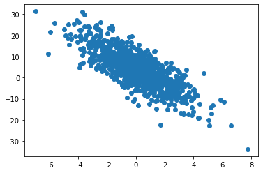
plt.scatter(features[:, 1], labels)
plt.show()

    true_param [ 2.6 -3.4  4.2]
​    features [[-1.64198071 -4.62281274  1.        ]
​     [ 4.99955694 -1.60475986  1.        ]
​     [-1.35368658 -2.47461838  1.        ]]
​    labels [[15.65474609]
​     [22.65296282]
​     [ 9.07303287]]

X = np.matrix(features) # 转换成矩阵计算
y = np.matrix(labels)
w = y.T * X * ((X.T * X) ** -1)
w

    matrix([[ 2.60006291, -3.39991021,  4.20011877]])

• 可以直接套用公式计算出近似解

梯度下降最小化$loss$ 函数

# 定义 loss 函数 (均方损失) 评价函数
def square_loss(y_hat, y, batch_size):
    # y_hat 可能是 (n,) 的张量而y 可能是 (n,1) 的张量
    return (y_hat - y.reshape(y_hat.shape)) ** 2 / (2 * batch_size)


# 定义模型
def linreg(X, param):
    return np.dot(X, param)

# 梯度下降优化函数 
# param 是一个行向量
# lr -> 学习率, batch_size -> 批个数
def sgd(param, labels, features, lr, batch_size):
    # 转成矩阵
    w = np.matrix(param).T
    y = np.matrix(labels)
    X = np.matrix(features)
    # 求梯度
    grad = - (1 / batch_size) * (y - (X * w)).T * X
    # 更新参数
    param -= lr * np.array(grad).reshape(param.shape)
    

# 测试一下
lr = 0.03
batch_size = sample_num # 全部训练集
# 初始化
param_test = np.array([1.6, -0.4, 2.2])

# 评估一下未训练前的均方损失
before = square_loss(linreg(features, param_test), labels, batch_size)

# 训练三次
sgd(param_test, labels, features, lr, batch_size)
sgd(param_test, labels, features, lr, batch_size)
sgd(param_test, labels, features, lr, batch_size)

# 再评估一次
after = square_loss(linreg(features, param_test), labels, batch_size)

print(f"before loss: {before.sum()}, after loss: {after.sum()} ")

    before loss: 20.79438217983131, after loss: 10.750752225581973 

• 对比未训练前，loss下降了一些，但依旧很大

加上随机小批量训练

# 定义随机小批量获取函数
def data_iter(batch_size, features, labels):
    num_samples = len(features)
    indices = list(range(num_samples))
    # 打乱索引
    random.shuffle(indices)
    
    # 确保每个 epoch 都能扫到所有的训练数据
    for i in range(0, num_samples, batch_size):
        batch = np.array(indices[i:min(i + batch_size, num_samples)])
        features_batch = features[batch]
        labels_batch = labels[batch]
        # 加上 batch 大小并返回
        yield features_batch, labels_batch, len(batch)
        

# 训练 10 次
epochs_num = 10

# 学习率
lr = 0.01

# 模型 -> 线性模型
net = linreg

# batch_size
batch_size = 10

# 定义 loss 函数
loss = square_loss

# 随机初始化
param = np.random.normal(loc=0.0, scale=0.01, size=3)

train_loss = []

def train():
    # 开始训练
    for epoch in range(epochs_num):
        for X, y, bs in data_iter(batch_size, features, labels):
            sgd(param, y, X, lr, bs)  # bs 是真实的 batch_size，防止训练集合数量不是 batch_size 的整数倍

        # 评估模型
        train_l = loss(net(features, param), labels, sample_num)
        print(f"epoch {epoch + 1}, loss {train_l.sum()}")
        train_loss.append(train_l.sum())
        
train()
print(f"param = {param}")

    epoch 1, loss 1.2065632092722889
​    epoch 2, loss 0.15898723733648745
​    epoch 3, loss 0.02137899866036004
​    epoch 4, loss 0.0028851708953185904
​    epoch 5, loss 0.00042819857542367157
​    epoch 6, loss 0.00010052808715963687
​    epoch 7, loss 5.779900635093226e-05
​    epoch 8, loss 5.1783731344928684e-05
​    epoch 9, loss 5.081713521527933e-05
​    epoch 10, loss 5.081523581349108e-05
​    param = [ 2.6003643  -3.39990574  4.19993823]

plt.plot(range(epochs_num+1)[1:], train_loss)
plt.show()

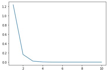
loss 在逐步下降，10 次训练后已经非常低了

• 但如果学习率取值不恰当，就会出现如下问题

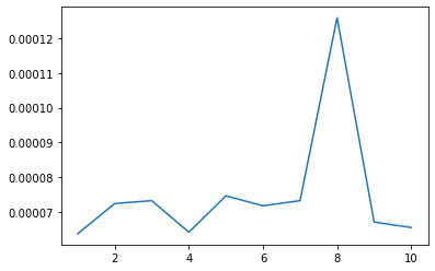
# 太大
lr = 0.3
train_loss = []
param = np.random.normal(loc=0.0, scale=0.01, size=3)

train()

plt.plot(range(epochs_num+1)[1:], train_loss)
plt.show()

    epoch 1, loss 6.379668827684062e-05
​    epoch 2, loss 7.248316610920411e-05
​    epoch 3, loss 7.329380803747091e-05
​    epoch 4, loss 6.425372957395597e-05
​    epoch 5, loss 7.468758571938891e-05
​    epoch 6, loss 7.182971239060776e-05
​    epoch 7, loss 7.330242279496708e-05
​    epoch 8, loss 0.00012583320290307138
​    epoch 9, loss 6.715234898209186e-05
​    epoch 10, loss 6.558175808855953e-05

# 太小
lr = 0.00001
train_loss = []
param = np.random.normal(loc=0.0, scale=0.01, size=3)

train()

plt.plot(range(epochs_num+1)[1:], train_loss)
plt.show()

    epoch 1, loss 43.83333313218246
​    epoch 2, loss 43.54262935003088
​    epoch 3, loss 43.254090728663186
​    epoch 4, loss 42.967700330914276
​    epoch 5, loss 42.68343716053708
​    epoch 6, loss 42.40129499586425
​    epoch 7, loss 42.12124256403142
​    epoch 8, loss 41.84327579643957
​    epoch 9, loss 41.56737663520067
​    epoch 10, loss 41.29352752241461

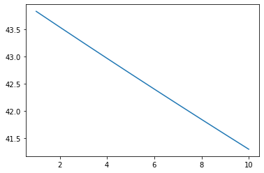
• 前者loss反复横跳，后者loss居高不下

使用 pytorch 自动求导

import torch

from torch.utils import data
from torch import nn

# 定义参数
batch_size = 10
# reshape 成二维张量再乘
true_w = torch.tensor([2.6, -3.4])
true_b = 3.2
sample_num = 1000


# 得到训练集
features = torch.normal(0, 1, (sample_num, len(true_w)))
labels = torch.matmul(features, true_w) + true_b
# 加上随机噪音
labels += torch.normal(0, 0.01, labels.shape)
labels = labels.reshape(-1, 1) # reshape 成列向量

# 得到 pytorch 的 dataset
dataset = data.TensorDataset(features, labels)

dataset = data.DataLoader(dataset, batch_size, shuffle=True)

# 这样就可以拿到 X, y
X, y = next(iter(dataset))
print(X[:3])
print(y[:3])

    tensor([[ 0.0210, -0.6603],
​            [-0.7817, -0.6642],
​            [-0.7901,  1.3997]])
​    tensor([[ 5.4977],
​            [ 3.4239],
​            [-3.6240]])

net = nn.Sequential(nn.Linear(2, 1))

net[0].weight.data.normal_(0, 0.01) # 权重
net[0].bias.data.fill_(1) # 偏差

    tensor([1.])

# 损失函数
loss = nn.MSELoss()

# 训练模型
trainer = torch.optim.SGD(net.parameters(), lr=0.03)

epochs_num = 3

for epoch in range(epochs_num):
    for X, y in dataset:
        # 求损失
        l = loss(net(X), y)
        # 梯度清零
        trainer.zero_grad()
        # 反向传递求梯度
        l.backward()
        # 更新模型
        trainer.step()
    
    # 评价
    l = loss(net(features), labels)
    print(f"epoch {epoch + 1}, loss {l:f}")
    
print(f"w = {net[0].weight.data}, b = {net[0].bias.data}")

     epoch 1, loss 0.000229
​    epoch 2, loss 0.000095
​    epoch 3, loss 0.000095
​    w = tensor([[ 2.5994, -3.3995]]), b = tensor([3.1995])